Build Proposal

Constructs the step optimized proposal density, squeezing function, and log-linear tail proposal for a user defined probability density function.

Usage

build_proposal(
  f,
  modes,
  lower = -Inf,
  upper = Inf,
  h = NULL,
  h_prime = NULL,
  steps = NULL,
  proposal_range = NULL,
  theta = 0.1,
  target_sample_size = 1000,
  verbose = FALSE,
  ...
)

Arguments

f: A function which returns the (unnormalised) probability density function of the target distribution. The first argument must be the value at which the pdf is to be evaluated. Additional arguments may be parameters of the distribution, which should be specified by name in the ... arguments.
modes: Numeric vector of modes of the density function.
lower: Numeric scalar representing the lower bound of the target density. Default is -Inf for unbounded lower support.
upper: Numeric scalar representing the upper bound of the target density. Default is Inf for unbounded upper support.
h: An optional function which returns the (unnormalised) log-probability density function of the target distribution. As for f the first argument must be the value at which the log-pdf is to be evaluated and additional parameters may be named arguments passed to ....
h_prime: An optional function which returns the first derivative of the (unnormalised) log-probability density function of the target distribution. As for f the first argument must be the value at which the log-pdf is to be evaluated and additional parameters may be named arguments passed to ....
steps: Optional integer scalar specifying the number of steps in the step optimised part of the proposal density and squeezing function.
proposal_range: Optional numeric vector of length 2 specifying the lower and upper range of the steps in the step optimised part of the proposal density and squeezing function. This range should be contained within the interval defined by lower and upper.
theta: Optional numeric scalar (between 0.1 and 1) defining the pre-acceptance threshold. This dictates when no further steps should be added in the step optimised part of the proposal density and squeezing function, based on the probability of pre-acceptance.
target_sample_size: Integer scalar indicating the typical sample size that will be requested when sampling from this density using build_sampler. The proposal optimization process bases benchmark timings on this target size in order to select a proposal best suited to the desired sample size. Note this does not limit sampling to this number, it is merely a guide should the user be aware that a certain sample size will be most commonly sampled.
verbose: Logical scalar. If TRUE, a table detailing the optimization areas and steps will be displayed during proposal optimization. Defaults to FALSE.
...: Further arguments to be passed to f, h, and h_prime, if they depend on additional parameters.

Value

This returns a list which is used to construct the sampler by passing to build_sampler function.

A list containing the optimized proposal and related parameters for the specified built-in distribution:

data

A data frame with detailed information about the proposal steps, including:

x: The start point of each step on the x-axis.
s_upper: The height of each step on the y-axis.
p_a: Pre-acceptance probability for each step.
s_upper_lower: A vector used to scale the uniform random number when the sample is accepted.

areas

A numeric vector containing the areas under:

left_tail: The left tail bound.
steps: The middle steps.
right_tail: The right tail bound.

steps_number

An integer specifying the number of steps in the proposal.

sampling_probabilities

A numeric vector with:

left_tail: The probability of sampling from the left tail.
left_and_middle: The combined probability of sampling from the left tail and middle steps.

unif_scaler

A numeric scalar, the inverse probability of sampling from the steps part of the proposal ($\frac{1}{p(lower < x < upper)}$). Used for scaling uniform random values.

lt_properties

A numeric vector of 5 values required for Adaptive Rejection Sampling (ARS) in the left tail.

rt_properties

A numeric vector of 6 values required for ARS in the right tail.

alpha

A numeric scalar representing the uniform step area.

tails_method

A string, either "ARS" (Adaptive Rejection Sampling) or "IT" (Inverse Transform), indicating the sampling method for the tails.

proposal_bounds

A numeric vector specifying the left and right bounds of the target density.

cnum

An integer representing the cache number of the created proposal in memory.

symmetric

A numeric scalar indicating the symmetry point of the proposal, or NULL if not symmetric.

f_params

A list of parameters for the target density that the proposal is designed for.

is_symmetric

A logical value indicating whether the proposal is symmetric.

proposal_type

A string indicating the type of the generated proposal:

"scaled": The proposal is "scalable" and standardized with rate = 1. This is used when parameter rate is either NULL or not provided. Scalable proposals are compatible with srexp.
"custom": The proposal is "custom" when rate is provided. Custom proposals are compatible with srexp_custom.

target_function_area

A numeric scalar estimating the area of the target distribution.

dens_func

A string containing the hardcoded density function.

density_name

A string specifying the name of the target density distribution.

lock

An identifier used for saving and loading the proposal from disk.

Details

This function is the starting point when a user wishes to build a custom sampler using StORS. It is responsible for generating the step optimized proposal density, squeezing function, and log-linear tail proposal that can be utilized for this purpose. The minimum information that must be supplied by the user is:

The (closed) interval of support for the distribution, [lower, upper] $\in \mathbb{R}$, which may also be half-closed on either side, or all of $\mathbb{R}$.
The probability density function (pdf), which need not be normalised, f.
Any modes of the pdf, as vector modes.

Optionally, the log-pdf and derivative of the log-pdf may be supplied.

Arguments for pdf

The pdf (and log-pdf and first derivative of the log-pdf) may depend on certain parameters. If so, these can be from the second argument onward in f. For instance, consider the Kumaraswamy distribution, which has pdf: $$f(x; a,b) = a b x^{a-1}{ (1-x^a)}^{b-1}, \ \ \mbox{where} \ \ x \in (0,1)$$ This pdf has known modes.

Then, to implement as a custom StORS sampler, we would first define the pdf in R:

dkumaraswamy <- function(x, a, b) a*b*(x^(a-1))*(1-x^a)^(b-1)

Then, to construct a StORS proposal for $a=2$ and $b=2$, we would call

Proposal <- build_Proposal(lower = 0, upper = 1, modes = sqrt(1/3), f = dkumaraswamy, a = 2, b = 2)

StORS proposal construction

StORS defines an unnormalised piecewise constant proposal density and squeezing function, with a Proposal defining the change points. To optimise the execution speed on modern CPUs, the unnormalised piecewise constant proposal has fixed area for each segment with one end of the segment coinciding with the user's pdf. That is, each step of the function has width defined by $w_i = (x_i - x_{i-1})$ and a height determined by $h_i = \max(f(x_{i-1}), f(x_i))$, such that $w_i h_i = \alpha \ \forall\,i$ where $\alpha$ is constant.

Once the user has constructed the proposal, the sampling function can be built using build_sampler().

Internal details

The function build_final_Proposal() manages the construction of these steps and calculates values critical for the sampling process. When the resultant Proposal is used with the build_sampler() function, these values are cached, significantly enhancing the computational efficiency and hence improving sampling speed. During the optimization process, we aim for a certain Proposal size based on L1-3 memory cache size. Therefore, we test the speed of Proposals of sizes $2^m$ Kb. To achieve this, we estimate the uniform step area based on a certain steps number that leads to the target cache size, $ \alpha = \frac{1}{\text{number of steps}} $.

The speed testing for each possible Proposal is initially based on a sample size of 1000. However, if the user wishes to optimize the Proposal for a different sample size, they can do so by specifying the desired sample size using the target_sample_size argument.

In case the user wants to select a specific number of steps for the proposal and bypass the optimization process, this can be done by specifying a steps number greater than the number of modes by 2 using the steps argument. If the target density is heavy-tailed, and the user wishes to stop the Proposal building process at a certain pre-acceptance threshold, this can be achieved by setting the acceptance probability threshold theta $\theta$. Once the steps reach this level of pre-acceptance probability, the step construction will end $ \frac{\min(f(x_i), f(x_{i+1}))}{\max(f(x_i), f(x_{i+1}))} < \theta $. Alternatively, if the user wishes to create the steps within certain limits on the x-axis, they can do so by specifying the proposal limits using the proposal_range argument.

Examples


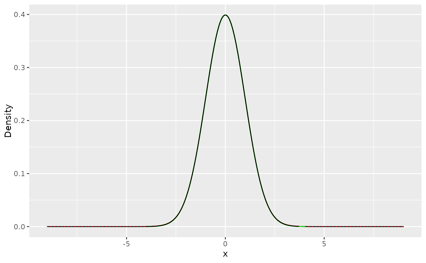
# Example 1: Building a proposal for Standard Normal Distribution
# This example demonstrates constructing a proposal for a standard normal distribution
# \( f(x) \sim \mathcal{N}(0,1) \),
# and shows the optimization table by setting \code{verbose} to \code{TRUE}.

# Define the density function, its logarithm,
# and its derivative for the standard normal distribution
modes_norm = 0
f_norm <- function(x) { 1 / sqrt(2 * pi) * exp(-0.5 * x^2) }
h_norm <- function(x) { log(f_norm(x)) }
h_prime_norm <- function(x) { -x }

# Following example takes slightly too long to run on CRAN.
# \donttest{
# Build the proposal for the standard normal distribution
norm_proposal = build_proposal(lower = -Inf, upper = Inf, mode = modes_norm,
 f = f_norm, h = h_norm, h_prime = h_prime_norm, verbose = TRUE)
#> 
#> ── Optimization Summary ────────────────────────────────────────────────────────
#> 
#> 
#>  Step:        Inf | Area: 0.008130081 
#> -----------------------------------------------
#>         Steps      |       Area       |    Best Sim Time
#>  -----------------------------------------------
#> ---        132 ---  --- 0.007723577 ---   ---  112741.00 ---
#> ---        126 ---  --- 0.008130081 ---   ---  126777.00 ---
#> ---        120 ---  --- 0.008536585 ---   ---  115240.00 ---
#> 
#> 
#>  Step:        Inf | Area: 0.003984064 
#> -----------------------------------------------
#>         Steps      |       Area       |    Best Sim Time
#>  -----------------------------------------------
#> ---        268 ---  --- 0.003784861 ---   ---   80766.00 ---
#> ---        254 ---  --- 0.003984064 ---   ---   74239.00 ---
#> ---        242 ---  --- 0.004183267 ---   ---   79974.00 ---
#> 
#> 
#>  Step:        Inf | Area: 0.001972387 
#> -----------------------------------------------
#>         Steps      |       Area       |    Best Sim Time
#>  -----------------------------------------------
#> ---        538 ---  --- 0.001873767 ---   ---   46176.50 ---
#> ---        512 ---  --- 0.001972387 ---   ---   59736.00 ---
#> ---        488 ---  --- 0.002071006 ---   ---   58013.00 ---
#> 
#> 
#>  Step:        Inf | Area: 0.000981354 
#> -----------------------------------------------
#>         Steps      |       Area       |    Best Sim Time
#>  -----------------------------------------------
#> ---       1078 ---  --- 0.000932287 ---   ---   36388.00 ---
#> ---       1024 ---  --- 0.000981354 ---   ---   32390.50 ---
#> ---        976 ---  --- 0.001030422 ---   ---   37941.00 ---
#> 
#> 
#>  Step:        Inf | Area: 0.000489476 
#> -----------------------------------------------
#>         Steps      |       Area       |    Best Sim Time
#>  -----------------------------------------------
#> ---       2156 ---  --- 0.000465002 ---   ---   26254.00 ---
#> ---       2048 ---  --- 0.000489476 ---   ---   19722.00 ---
#> ---       1952 ---  --- 0.000513950 ---   ---   28418.00 ---
#> 
#> 
#>  Step:        Inf | Area: 0.000244439 
#> -----------------------------------------------
#>         Steps      |       Area       |    Best Sim Time
#>  -----------------------------------------------
#> ---       4312 ---  --- 0.000232217 ---   ---   19401.50 ---
#> ---       4098 ---  --- 0.000244439 ---   ---   19361.00 ---
#> ---       3902 ---  --- 0.000256661 ---   ---   18780.00 ---
#> 
#> 
#>  Step:        Inf | Area: 0.000122145 
#> -----------------------------------------------
#>         Steps      |       Area       |    Best Sim Time
#>  -----------------------------------------------
#> ---       8626 ---  --- 0.000116038 ---   ---   19261.00 ---
#> ---       8194 ---  --- 0.000122145 ---   ---   14166.50 ---
#> ---       7804 ---  --- 0.000128252 ---   ---   16701.50 ---
#> 
#> 
#>  Step:        Inf | Area: 0.000061054 
#> -----------------------------------------------
#>         Steps      |       Area       |    Best Sim Time
#>  -----------------------------------------------
#> ---      17248 ---  --- 0.000058001 ---   ---   25653.00 ---
#> ---      16386 ---  --- 0.000061054 ---   ---   25196.50 ---
#> ---      15606 ---  --- 0.000064106 ---   ---   18780.00 ---
#> 
#> ────────────────────────────────────────────────────────────────────────────────
#> 
#> ── Performance Data: ───────────────────────────────────────────────────────────
#>      Area       |     Time     |   Steps
#> -----------------------------------------
#>  0.0077235772 |  112741.00 |     132
#>  0.0039840637 |   74239.00 |     254
#>  0.0018737673 |   46176.50 |     538
#>  0.0009813543 |   32390.50 |    1024
#>  0.0004894763 |   19722.00 |    2048
#>  0.0002566610 |   18780.00 |    3902
#>  0.0001221449 |   14166.50 |    8194
#> ────────────────────────────────────────────────────────────────────────────────

# Plot the generated proposal
plot(norm_proposal)

# }

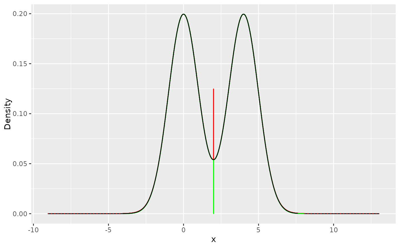
# Example 2: proposal for a Bimodal Distribution
# This example shows how to build a proposal for sampling from a bimodal distribution,
#combining two normal distributions
# \( f(x) = 0.5 \cdot w_1(x) + 0.5 \cdot w_2(x) \),
# where \( w_1(x) \sim \mathcal{N}(0, 1) \) and \( w_2(x) \sim \mathcal{N}(4, 1) \).

# Define the bimodal density function
f_bimodal <- function(x) {
  0.5 * (1 / sqrt(2 * pi)) * exp(-(x^2) / 2) + 0.5 * (1 / sqrt(2 * pi)) * exp(-((x - 4)^2) / 2)
}
modes_bimodal = c(0.00134865, 3.99865)

# Build the proposal for the bimodal distribution
bimodal_proposal = build_proposal( f = f_bimodal, lower = -Inf, upper = Inf, mode = modes_bimodal)

# Print and plot the bimodal proposal
print(bimodal_proposal)
#> 
#> ── Proposal Summary ────────────────────────────────────────────────────────────
#> • Total steps: 7,806
#> • Steps range: [-4.044247, 8.042763]
#> • Sampling efficiency: 99.88%
plot(bimodal_proposal)


# Example 3: Proposal with 500 Steps for Bimodal Distribution
# This example demonstrates constructing a proposal with 500 steps,
# for the bimodal distribution used in Example 2.

bimodal_proposal_500 = build_proposal(f = f_bimodal, lower = -Inf, upper = Inf,
 mode = modes_bimodal, steps = 500)

# Print and plot the proposal with 500 steps
print(bimodal_proposal_500)
#> 
#> ── Proposal Summary ────────────────────────────────────────────────────────────
#> • Total steps: 500
#> • Steps range: [-2.332842, 6.332824]
#> • Sampling efficiency: 98.89%

Usage

Arguments

Value

Details

See also

Examples